The predictions from housing theory are:
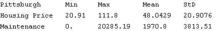
Here are the descriptive statistics for each city. Housing price is price per square foot. Maintenance includes renovation work.
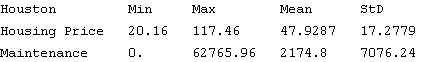
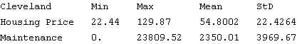
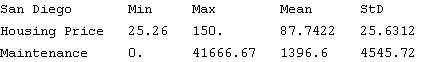
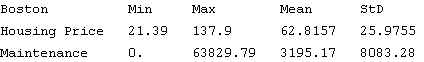
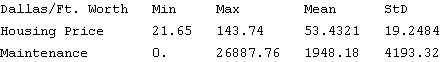
You may notice that the home values in older cities have a slightly wider variation of prices compared to the newer cities (Cleveland is the exception). Part of this is due to a wider variations in types and ages of homes. Of the six metropolitan areas, San Diego has the highest mean value of $87.74 /sq. foot (compared to $47.93 for Houston, the city with the lowest mean). A 2,000 square foot home that is "typical" within each market ranges in estimated value from $95,860 (in Houston) to $175,480 (in San Diego).
It is true that lower quality homes are valued less than higher quality homes. In some urban housing markets, there is a negative correlation between housing quality and age. This implies that older homes are lower quality and therefore, are valued less. The relationship between age and quality does not hold for many markets, there are plenty of examples of older homes in the Boston, Baltimore, San Francisco, New York and Chicago housing markets that are highly valued.
Maintenance has the greatest variation. In examining the Max values, it is clear that the cost reported can include major renovation or repair. The Min value is zero for all markets - for some years, it is expected that a homeowner will not incur any maintenance costs.
Differences between cities
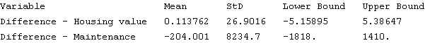
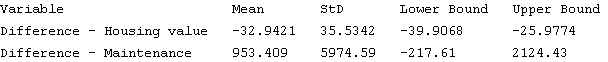
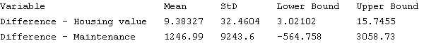
A number of conditions contribute to the relationship between age and quality - too many to mention here. Answers for questions 1 & 2 are given below. "Lower Bound" is the lower bound value of the confidence interval, "Upper Bound" is the upper bound value.
With respect to differences in home values, the only data set that shows the predicted results is the data set of Cleveland and San Diego. Cleveland homes, on the average, are $33.00 per square foot less than San Diegos'. The opposite outcome is found with the data set containing data from Boston and Dallas/Ft. Worth. On the average, the sample homes in Boston cost $9.40 per square foot more than in Dallas/Ft. Worth. As one can see, there is very little difference between the price per square foot for homes in Pittsburgh and Houston. The mean difference in prices is less than 25 cents/sq. foot.
The confidence intervals tell you something about the expected population value (e.g., difference in the population means of home values). For Boston and Dallas/Ft. Worth, the interval is a range of positive values (3.02 to 15.75). This tells you that, with 95% confidence, the true parameter is positive, that is, it is fairly certain that Boston's prices are higher. The confidence interval for Cleveland and San Diego is negative (-39.91 to -25.98). With 95% confidence, one can say that Cleveland's home values are lower than San Diego's. The confidence interval for Houston/Pittsburgh is nearly evenly divided between positive and negative values - this implies that the true difference in home values can go either way.
Pittsburgh and Houston
Cleveland and San Diego
Boston and Dallas/Ft Worth
With respect to maintenance, the mean differences in the Cleveland/San Diego and Boston/Dallas-Ft Worth markets are consistent with the prediction of theory (e.g., older homes cost more to maintain). The Houston/Pittsburgh markets report the opposite outcome.
The confidence intervals for the population parameter (difference in means) tell you that the true difference in means can be negative or positive. There appears to be no pattern between the age of the cities and housing maintenance.
Hypothesis test - Older homes are valued less than newer homes.
Are older homes valued less than newer homes? To test this, we first set up the null hypothesis

where older and newer refer to old and new cities.
The alternative hypothesis is

Based on the null and alternative hypotheses, we use a one-tailed
test. Analysis is bivariate, sample size is large (n=100), variable is interval so we use
the Sample Test of the difference in means - large sample.
With respect to the distribution of z scores, the rejection region for this problem lies in the right tail. Large, positive z scores will reject H0. Using the table from the handout, here is a list of rejection values.
| p value | Z values greater than this will reject H0. |
| p=0.10 | 1.28 |
| p=0.05 | 1.645 |
| p=0.01 | 2.33 |
Here are the outcomes for the three projects
Houston and Pittsburgh

Cleveland and San Diego

The report from mathematica is wrong. Test Statistic that rejects the null is positive.
Boston and Dallas/Ft Worth

The report from mathematica is correct. Test Statistic that rejects
the null is positive.
This table summarizes the outcomes.
| Cities | p values | Reject/Fail to reject |
| Pittsburgh/Houston | p=0.10 | Fail to reject |
| p=0.05 | Fail to reject | |
| p=0.01 | Fail to reject | |
| Cleveland/San Diego | p=0.10 | Fail to reject |
| p=0.05 | Fail to reject | |
| p=0.01 | Fail to reject | |
| Boston/Dallas-Ft Worth | p=0.10 | Reject |
| p=0.05 | Reject | |
| p=0.01 | Reject |
Hypothesis test - Older homes cost more to maintain than newer homes.
The null hypothesis is:

with the alternative hypothesis

The null hypothesis states that the population distributions of older and newer cities are different and that the mean maintenance value for homes in older cities is greater than homes in newer cities.
This is a one-tailed test. Below are the rejection regions. Z scores that reject the hypothesis are very small and negative - they are found in the left tail region of the distribution.
| p value | Z values less than this will reject H0. |
| p=0.10 | -1.28 |
| p=0.05 | -1.645 |
| p=0.01 | -2.33 |
Here are the results
Houston and Pittsburgh

Cleveland and San Diego

Boston and Dallas/Ft Worth

Here are the results in table form
| Cities | p values | Reject/Fail to reject |
| Pittsburgh/Houston | p=0.10 | Fail to reject |
| p=0.05 | Fail to reject | |
| p=0.01 | Fail to reject | |
| Cleveland/San Diego | p=0.10 | Fail to reject |
| p=0.05 | Fail to reject | |
| p=0.01 | Fail to reject | |
| Boston/Dallas-Ft Worth | p=0.10 | Fail to reject |
| p=0.05 | Fail to reject | |
| p=0.01 | Fail to reject |
The Houston/Pittsburgh data is the only set of data that generated a negative z score. This z score (-0.255) doesn't fall in the rejection range. The data does not support the rejection of the null hypothesis. There is no support from the data to reject the hypothesis that homes in older cities cost more to maintain than homes in newer cities.
Conclusion
What can we say about the overall results? Only one set of cities (Boston/Dallas-Ft. Worth) shows results that are contrary to the prediction from theory that homes in older cities are valued less than homes in newer cities. Data from the other cities show results that are not contrary. Maintenance data results do not reject the prediction that homes in older cities cost more to maintain that homes in newer cities.
Appendix: can we go beyond these results?
Yes. We can run two-tailed hypothesis tests to determine if the population means for home value and maintenance are the same for older and newer cities. We can also run the one-tailed test to determine if the population means for home value is greater for older cities and the maintenance cost is less for older cities.
Specific Sample tests are not given but the results from these tests are summarized below. The columns marked as "primary tests" are the results given above.
| Cities | Prediction: Differences in home values - old and new cities | Prediction: Differences in maintenance cost - old and new cities | ||||
| Homes in older cities are valued the same as in newer cities | Homes in older cities are valued more than in newer cities. | Homes in older cities are valued less than in newer cities. (primary tests) | Maintenance cost for homes in older cities is the same as in newer cities. | Maintenance cost for homes in older cities is higher than in newer cities. (primary tests) | Maintenance cost for homes in older cities is lower than in newer cities. | |
| Pittsburgh/Houston | Fails to reject prediction | Fails to reject prediction | Fails to reject prediction | Fails to reject prediction | Fails to reject prediction | Fails to reject prediction |
| Cleveland/San Diego | Data rejects prediction at p=.10, .05 and .01 | Data rejects prediction at p=.10, .05 and .01 | Fails to reject prediction | Fails to reject prediction | Fails to reject prediction | Data rejects prediction at p=.10 |
| Boston/Dallas-Ft Worth | Data rejects prediction at p=.10, .05 and .01 | Fails to reject prediction | Data rejects prediction at p=.10, .05 and .01 | Data rejects prediction at p=.10 | Fails to reject prediction | Data rejects prediction at p=.10 |
Boston/Ft.Worth
Shows the strongest results - based on rejected predictions, this combination of cities describe one type of relationship, there exist cities in the US with older housing stock that are highly valued. Maintenance is high because it is a proportion of the value of the home.
Cleveland/San Diego
Shows strong results supporting the prediction that the value of homes in older cities are less than the value of home in newer cities - provides some support for the maintenance prediction, data rejects the prediction that older homes cost less to maintain.
Pittsburgh/Houston
Information provides no direct support for either of the two predictions.
Further Research
Could look at other combinations of cities - could examine within characteristics of the city to see if other factors matter. With respect to maintenance cost, based on my research of owner-occupied homes in the US, I have found that the following factors matter.
- Age of structure - maintenance cost rises for structures between the age of 0 (new homes) and 15 years - cost remains constant for homes that are older than 15 years. Perhaps older homes that are more costly to maintained are removed from the housing market or converted into rentals.
- Tenure (how long the owner has lived in the home) - very little maintenance cost initially - rises as the tenure period increases. This result hold for households who purchase new and old structures.
- Owner's wealth - wealthier homeowners take on a higher level of maintenance.
- Estimated value of the home - homeowners put a higher level of maintenance into high valued homes.
- Size of the structure - Larger structures have higher maintenance costs.
- Quality of the neighborhood - Homeowners put higher levels of maintenance in neighborhoods they perceive as low quality - perhaps they offset poor quality public services for more private services. Perhaps people with strong concerns for neighborhood quality have strong concerns about the quality of their homes.
- Age of the homeowner - level of maintenance is lower for older homeowners.
What is also important is to look at the factors that do not matter.
- Lotsize
- Race