A. Introduction to Arena Simulation [SS]

Simulation is one of the most powerful analysis tools available to those responsible for the design and operation of complex processes or systems. In an increasingly competitive world, simulation has become a very powerful tool for the planning, design, and control of systems. No longer regarded as the approach of “last resort” it is today viewed as an indispensable problem-solving methodology for engineers, designers, and managers [7].

This article presents some important features of the ARENA 3.0 software. This would help the beginner to understand the basic concepts necessary for building a simple model. This in turn could provide a springboard for building up complex real world models.

A Simple Simulation Model

Let us consider a simple simulation model. Suppose we have a single-channel queuing (waiting line) system, such as a checkout counter in a drugstore. The time between the arrival of customers is uniformly distributed from 1 to 10 minutes. This is obtained by means of a spinner dial (such as those used in some board games). The time required to service a customer be uniformly distributed between 1 to 6 minutes. A single die can be used to generate service times. The system has two random variables and if a large number of readings need to be generated, a computer is needed for generating the random variables and for doing the bookkeeping. To simulate real-world systems adequately, we must also be able to generate behavioral characteristics that are realistic. For example, the time between arrivals and the service times generated must allow for something other than uniform distribution rounded to the nearest whole number [7].

Distribution Selection

To test the compatibility of a set of observed frequencies with some theoretical frequency, we must first identify the theoretical distribution we wish to try. If we are dealing with a discrete variable, we record the frequency occurring within which each individual value occurs. If the variable is continuous, we break the range of values into equal interval or class. The relative frequency in each interval is then the observed frequency count in each class divided by the total number of data points [7].

After we have obtained a relative frequency distribution, selecting the possible probability distribution from which it may be derived becomes a matter of judge and experience [7].

Some examples of continuous distributions are uniform, triangular, negative exponential, Erlang, gamma, Weibull, normal, lognormal, and beta. Some examples of discrete distributions are discrete uniform, binomial, geometric, and Poisson [7].

Goodness-of-Fit Test

Once we have selected a distribution (based on visual inspection and theoretical grounds), we then need to assess the quality of our fit. This can be done by using formal statistical tests or by employing a simple graphical method in which an overlay of the theoretical distribution is displayed on a histogram of the data and a visual assessment is made to determine the quality of the fit. A goodness-of-fit test attempts to measure and evaluate the deviation of the sample distribution from the theoretical. Examples of these tests include both the Chi-Square (x^2) and the Kolmogrov-Smirnov tests [7].

Basic Modeling Concepts

IN ARENA3.0 environment, the word "entity" is a generic term used to denote any person, object, or thing- whose movement through the system causes change in the state of the system. Every entity possesses some unique characteristics referred to as attributes . For example in a factory a job may have attributes specifying the part number, due date, and priority of the job. The term variables, refers to the set of changeable values characterizing the components of the system as a whole. Example of a variable is TNOW. It specifies the current value of the simulated time [8].

In the ARENA3.0 modeling framework, there is a fundamental distinction between the Model and the Experiment. The model is a functional description of the system’s components and their interactions. The experiment defines the experimental conditions under which the model is exercised to generate specific output data. An ARENA3.0 simulation program generates both a model and corresponding experiments [8].

Processes are modeled in SIMAN by using a block diagram. A block diagram is a flow graph depicting the process through which the entities in the system move. The block diagram is constructed as a sequence of blocks, the shapes and names of which indicate their general function. The experimental section of the program consists of elements which, are specified interactively in the Arena modeling environment [8].

Blocks
The following section describes in brief the different blocks used by the simulation team.

CREATE: It is one of the several mechanisms by which an entity (product) can enter into the model. It is typically used to model arrival processes in which entities sequentially enter the model according to a specified pattern. The operands of Create block are Batch size indicating the number of entities arriving simultaneously in the model, Offset time specifying the time between the start of simulation and the arrival of the first entity, Interval specifying the delay between the arrivals at successive points after the first. The Maximum Batches operand specifies the maximum number of arrival points [8].

QUEUE: It provides waiting space for the entities whose movements through the model have been suspended based on the system’s status. An example is a work piece Waiting in turn to be processed on a busy machine. The operands of queue block are Queue ID indicating the name of the queue, Capacity of the queue and the Balk label which is used to direct the entity to an alternative block other than the seize block [8].

SEIZE: It is used in conjunction with the queue block and is used to model the status delays. When a resource becomes idle the entity from the previous queue block enters the seize block and seizes the resource. The state of the resource now changes from idle to busy. The operands of seize block include priority for the allocation of entities waiting for the same resource. Priority is given to those entities, which have been waiting the longest. The Resource ID indicating the resource requested by the waiting entity and the number of units of the resource requested by the entity [8].

DELAY: Once an entity has been allocated the necessary resources, it typically engages in time-consuming activities, such as setup, machining, inspection etc. In ARENA3.0, delays such as these can be modeled by using the DELAY block. The operands of the delay block are the duration of the delay and the storage ID, which provides statistics on the number of entities residing in one or more DELAY blocks [8].

RELEASE: When an activity that requires resources has been completed, the entity possessing the resources typically releases them so that they can be allocated to entities either currently waiting or yet to arrive at QUEUE-SEIZE blocks. Operands of seize block are Resource ID indicating the resource just released and the Quantity of entities to release simultaneously [8].

COUNT: It is used to count the number of occurrences of some event, e.g., work-pieces entering the system, exiting the system or sent through rework. The operands of the Count block include the Counter ID (name of the counter) and the Counter increment for which, a default value of one is assumed [8].

DISPOSE: It provides a mechanism for modeling the departure of entities from the system. The dispose block has a single entry point, no operands, and no exit points. All entities entering the dispose block are terminated from the model [8].

GROUP: It is commonly used to group a set of entities having a particular set characteristics. A representative entity is created and it moves through the model and behaves, as though, it is a single entity. The most important operand of group block is the quantity to group. This is commonly used to simulate a manufacturing scenario in which a set of parts corresponding to a particular product need to be grouped before they can be assembled by the machine [8].

SPLIT: The entities, which had been grouped, need to be split or de-grouped before they are disposed. The split block is used for the same. The departing entities have the original attribute values they had when the entity set was formed [8].

ASSIGN: Whenever attributes and variables are used in a model they need to be assigned values during model execution. This is made possible by means of the assign block. The operand of the block is Variable or Attribute = Value. Each time an entity passes through the ASSIGN block, the value on the right hand side of the equals sign is copied on to the variable or attribute on the left hand side of the equation. Example when the entities pass through the CREATE block they can be assigned a job type of 1,2,3 with a certain probability of the entity belonging to each type [8].

BRANCH: This is used to direct the entities to different sections of the model depending upon the condition of true or false. The operands of the branch block are the following:

1. Maximum Number of Branches (it is usually 1).
2. With (indicates the probability and the label to which the entity needs to be directed).
3. Else (indicates the label to which the entity needs to be directed if the else condition becomes true).
4. Always (whatever the condition the entity needs to be sent to a specific label).

Elements
The following section describes in brief the various elements used by the simulation team in developing the project.

PROJECT: It is used to describe the simulation project used by ARENA3.0 in labeling the SIMAN summary report. The program automatically generates this report at the end of each replication if it is defined under the experimental conditions. The operands of the element include Project Title, Analyst Name, Date, Summary Report (yes/ no). Maximum of 24 characters can be entered in the first two fields [8].

QUEUES: It defines the information of the model’s queues. The operands of the queue element are Number (need not be defined), Name of the queue, Ranking Criterion . The following criterion are used:

1. FIFO (First-in, First-out): Entities wait in the queue in the order in which they arrive.
2. LIFO (Last-in, First-out): Entities are ranked in the reverse order of their entry into the queue.
3. LVF (Attribute ID): The queue is ordered by increasing values of the specified attribute with ties broken by the FIFO rule.
4. HVF (Attribute ID): Queue is ordered by the decreasing values of the specified attribute with ties broken by the FIFO rule [8].

COUNTERS: This element provides descriptive information of the counters included in the model section. The operands included in the element are Number (need not be defined), Name of the counter, Limit. The last operand specifies a certain value which when exceeded causes the program to terminate [8].

REPLICATE: It defines the Number of Replications for which the simulation is to be run, the Beginning Time of the first replication and the Replication Length, which defines the duration of each simulation replication [8].

ATTRIBUTES: and VARIABLES: These elements provide general information about the symbolic names and properties of the attributes and variables. The operands of the elements include Number (optional), Name (index), Initial Values. The second operand is used to specify an array with certain index values. Each element in the array has a unique index value, which is stored in a common array name. The third variable is used to initialize a variable to a certain value [8].

STATIONS: It defines the information of the stations used in the model. The operands include Number (optional), Name of the station [8].

SETS: It defines a group of similar elements that may be referenced by a common name and set index. The elements that make up the set are referred to as the members of the set. Typical sets would contain groups of resources, queues, stations, pictures, counters, tallies, expressions, etc. The operands of the element are Number (optional), Name of the Set and the Members of the set. The last operand can be referenced by the set name. The function used by the Simulation team in building the manufacturing model was MemIdx (Setname, Member Name). This function returns the index number of a specific member in the set. The member name was the first station at which the entity entered the model [8].

SCHEDULES: This is used to change the capacity of the resource over time. The resource follows a time dependent schedule as specified in the element. For example, the resource is idle for the first 30 minutes of the simulation run. During this period it has a capacity of 0. During the next 30 minutes of the run the resource can have a capacity of 1. The operands of the element include Identifier, which is fed into the resource block following the schedule and Resource Capacity and the Capacity Duration, which specifies the capacity of the resource during a certain time period [8].

SEQUENCES: It defines the sequence in which an entity visits the stations. The operands include Number (optional), Name of the sequence, Station ID and the Assignments (duration of delay, assignment of picture or job type, etc.) at each station [8].

Arena3.0 Verification Tools Used by the Simulation Team

1. RUN CONTROLLER: It allows the user to step through the execution of the model by exercising complete control from the keyboard or the mouse. The entity can be moved through one or more blocks, its value can be examined by using simple commands. The execution can also be suspended at critical points or when specified variables reach defined values. The run controller also provides access to a model’s source statements, which can be listed during execution [8].

2. ANIMATION: Successful verification depends on one’s ability to comprehend the complex interactions among the many components within a model. Of all the techniques available to help in the verification process, animation is without a doubt the single, most powerful aid available. Only animation can present a dynamically moving picture of the many interactions taking place within the simulation. The animation displays the same information for all model components simultaneously [8].

Back to Table of Contents

 B. Computer Manufacturing Model [LR]

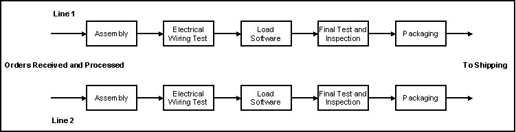
The computer manufacturing model differs from the automobile model with regards to detail, layout, and input data. Less detailed than the automobile manufacturing model in terms of specifying individual operations in the assembly stage, the computer manufacturing model simulates five main stages in assembling and testing computers. These processes are:

1. Assembly
2. Electrical testing
3. Software loading
4. Final testing and inspection
5. Packaging

Each line is analagous to a work cell in that material flows continuously through each stage with minimal in-process inventories. A complete product is manufactured at each cell, which uses equipment for each stage of the production process.

As described in the Manufacturing Team's web site, a typical manufacturing plant consists of four main components:

• Receiving
• Production Processing
• Packaging, and
• Shipping

Receiving
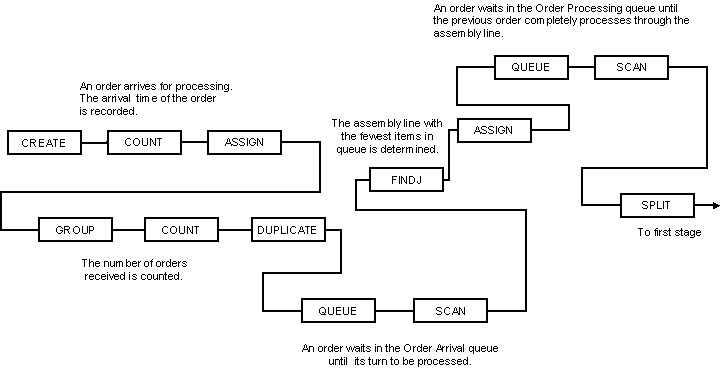
Orders of varying sizes arrive in intervals and are processed as first-in-first-out. For simplification, all requested computers in a particular order have the same configuration. The configuration consists of processor type, number of boards, and monitor type. The model specifies three types of processors, two types of boards, and two types of monitors. These attributes are probalistically assigned to each order with 12 configurations possible. Orders are sent to the least busy line but wait to be filled until the assembly stage is free. The model assumes that all raw materials for the assembly stage are readily available and are sufficient to fill each order. The logic for order processing in Arena is shown below.

Production Processing and Packaging
As mentioned previously, the production layout consists of two repetitive parallel lines. Orders are fed to each line, which consists of five stages. The processing times for each stage are: assembly - 12 minutes, electrical wiring test - 5 minutes, load software - 15 minutes, final test and inspection - 5 minutes, and packaging - 5 minutes. The utilization rate of the assembly stage is driven by the nature of the orders arriving: the size of each order and the time between orders. Queue formations and potential bottlenecks may occur at the assembly and loading software stages, where the processing times are high. These problems may be addressed by increasing the capacity of the resources, such as adding a third assembly stage or loading software for multiple computers at a time. Packaging involves selecting the appropriate monitor for the order and sending the packages to the shipping area.

Shipping
Although the computer model does not specifically simulate shipping activities, the model is flexible enough to have this component included at a later date. One consideration may involve combining packaging and shipping activities into one area.

The input data for the computer manufacturing model was not obtained from actual existing data from any particular computer manufacturer. Instead educated guesses were made for order sizes and processing times. Although one of the tenets in developing any simulation model involves obtaining actual data, this requirement was lifted in order to show a simple manufacturing model that utilizes parallel manunfacturing cells, and how the sizes, arrival, and number of orders affect assembly utilization rates.

Back to Table of Contents

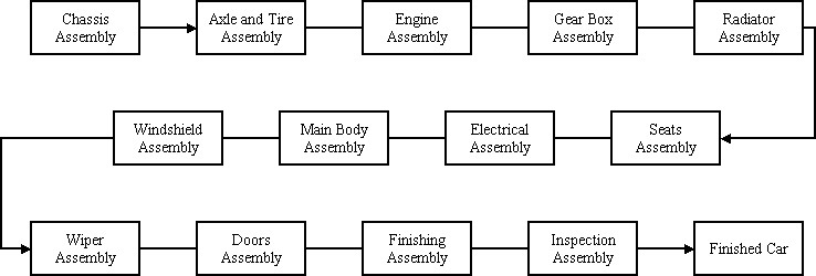
 C. Automobile Manufacturing Model [AB]

The automobile is perhaps the most important invention second only to electricity in the 20th century. It has changed life of man in a way unimaginable before its invention. "The world travels on wheels" is the buzzword of the 20th century. The manufacturing of these automobiles is both a fascinating and challenging task. The simulation team has simulated the manufacturing process of wagons, sedans and convertibles in a Toyota car plant.

The following is the step by step procedure for the manufacturing of cars in the "Toyota Production System":

1. The manufacturing process begins with the chassis assembly. The chassis is the skeleton of the car. It is the part on which the car is built.
2. Axle and tires are fitted to the chassis assembly.
3. In the next stage, the engine is fitted to the chassis. The engine is the power-producing component of the car. The power produced in the engine is use to propel the car. Engines are mostly of the internal combustion type.
4. The gearbox is then fitted into the chassis. The gearbox is the component that is used to change the speed supplied to the wheels.
5. The next stage involves the fitting of the radiator into the engine. The radiator helps in cooling the engine, transmitting the excess heat to the surrounding by conduction.
6. The seats are then fitted to the car in the next stage.
7. The battery is then fitted and electrical connections are carried out. The electrical connections connect the various components of the car to the battery.
8. The body of the car is then fitted on the chassis.
9. The windshield, doors, and wipers are fitted to the car along with the bonnet.
10. The finishing touches are carried out on the car.
11. The car is then sent for inspection and testing after which it is taken to the parking lot and kept ready for shipping.

The student version of the model limited the number of blocks to be used. The challenge was to use the limited number of blocks available without simplifying the process. For this purpose Sets were used along with Attributes such as "Work time" and "Op time." Given below is a brief explanation of attributes, variables, sets and counters used in the model.

Attributes

1. Worktime: If the job arriving at the workstation is a Hardtop or a Wagon it is delayed by the duration given in the work time attribute of the delay block.
2. Optime (operation time): If the job arriving at the workstation is a Sedan it is delayed by the duration given in the Op time attribute of the delay block.
3. Setindex: Corresponds to a specific workstation in the set of stations.
4. Timein (time in): Denotes the time at which a job arrived in the system.
5. Jobtype (type of job): Denotes that the type of job is a hardtop, wagon or sedan.

1. Queueset: Signifies all the queues along the main assembly line, which are sequentially visited by the job.
2. Stationset: Corresponds to all the stations along the main assembly line, which are sequentially attended by the job.
3. Resourceset: Denotes all the resources along the main assembly line, which are sequentially attended by the job.

1. Wagons: Number of wagons produced
2. Hardtops: Number of hardtops produced
3. Sedans: Number of Sedans produced
4. Total cars: Total number of cars produced

1. Mean
2. C
3. Std

Back to Table of Contents

 D. Transportation Model [AT]

For any organization having several manufacturing facilities, and a huge and spread market, transportation remains an inevitable part of its total system. The transportation model developed by the simulation team serves as a guideline to study how automobiles manufactured at a particular facility are transported to various places.

Following is a brief procedure on how this transportation takes place:

1. At first all the cars are accumulated in a huge parking lot, which also serves as a loading area for the trucks that carry these cars.
2. Once the specified number of cars is available, they are loaded on to the trucks as per the capacity of the trucks.
3. These trucks then transport the vehicles to the specified destination, such as a dock, where all these trucks are then handed over to a distributor.
4. At the dock, the vehicles are unloaded from the trucks, and then loaded onto a ship.
5. Once the ship is loaded to its capacity, it is then directed to its destination, which may be other countries, or within the nation, but to different states.

The attributes, variables, sequences, etc. that are used in the model are explained below:

Attributes: Time-In is the only attribute used in the model, which determines what time the car entered the system, for how long it was in the system.
Schedules: This element describes the schedules for the resources, when they are available and when they are not.
Counters: Counts the total number cars that are transported during the specified time.
Transporters: There are two types of transporters, Trucks and Ship, which are being used in this model.

Back to Table of Contents