How to Make a Tree

There is a major defect with the truth table method for determining whether an argument is valid. When there are many different letters in an argument, the number of rows in the truth table can be very large. Since the number of rows doubles with each added letter (for 2 letters - 4 rows, 3 letters - 8 rows, 4 letters - 16 rows, etc..) the table contains more than a thousand rows for an argument with only 10 letters. The tree method is a variation on the truth table method which can vastly shorten validity calculation. True, a tree may take as long as the corresponding table in the worst case, but the chances are very good that it will yield massive savings in effort.

The main idea behind the tree method is to avoid calculating any parts of the table which do not contribute to the main objective in the validity test, namely to find a row where all the premises are T and the conclusion is F. If there is such a row, the argument is invalid, because validity requires that it is impossible for (all) the premises to be T and the conclusion F. Let us call a row with (all) T premises and a F conclusion a counterexample. The idea behind tables is to examine all possible combinations of truth values to see whether there is a counterexample. If there is, the argument is invalid, and if not, it is valid. The tree method is more economical than tables because it calculates only those portions of the table where a counterexample can be. To help illustrate the point, consider this table for the following invalid argument: Q>-P | P>Q.

Note that the third row is a counterexample to the argument - it shows that the argument is invalid because it is possible for the premise to be T and the conclusion F. If we had some way to know to calculate only this third row, and to ignore the other three, we would have the answer (invalid) with only 1/4 the effort.

So let us see whether we can find a method to locate rows where counterexamples will be. Suppose that the argument Q>-P | P>Q does have a counterexample. Then there must be a row where Q>-P is T and P>Q is F. But there is only one way for a conditional like P>Q to be F, namely when the antecedent (P) is T and the conclusion (Q) is F. This means that if there is a counterexample at all, it must be on the row with P = T and Q = F, i.e. the third row. No other rows could possibly count as a counterexample, because on these rows the conclusion will be T. At this point we can easily check that the premise Q>-P is indeed T on this row, verifying that row 3 is indeed a counterexample.

Notice how this reasoning focuses our attention on the crucial third row, and helps us see why it is pointless to calculate out the other three rows. By reasoning backwards from the fact that a counterexample requires an F conclusion to the values the letters must have, it may be possible to narrow down a search for a counterexample to one or two rows. (The same idea may also be used on the premises: knowing that a premise has to be T, also yields information on what values the letters have to have in a counterexample.)

You may get the impression that this idea only works for invalid arguments where a counterexample exists. But it works for valid arguments as well. Let us use P>-Q | Q>-P to illustrate. If this argument were to have a counterexample, then there would have to be a row where P>-Q = T and Q>-P = F. From the latter fact, it follows that the row would have to have Q = T and -P = F. There is only one row like this, namely where Q = T and P = T. But if this row is a counterexample it must make P>-Q = T. However, it does not, since P = T and Q = T makes -Q = F, with the result that P>-Q = F. The only possible counterexample to our argument is the row where P = T and Q = T. But we have just seen that it does not make the premise T, so it does not qualify as a counterexample. It follows that the argument has no counterexample, and so it must be valid. Notice that even in the case of this valid argument, we only needed to consider calculating out values for one of the four rows.

So far we have only explained ideas behind the tree method. It is time to learn the notation and details. The basic idea is to develop a coordinated search for a counterexample to our argument by using the information that the premises must be T and the conclusion F. One notation for doing this involves labeling formulas and their parts with Ts and Fs to indicate their values. However, this can be both conceptually and visually confusing. Instead, the tree method uses the convention that every sentence we write down is considered to be T. If we want to indicate that sentence P is F, we simply write down -P instead, (for if -P is T, P must be F). Let us illustrate this idea by actually building the tree for the argument P>-Q | Q>-P. We begin with the information that if the argument is to have a counterexample in some row, then P>-Q must be T and Q>-P must be F:

P>-Q

-(Q>-P)

Note that to indicate Q>-P = F, we have written -(Q>-P) instead. Now if -(Q>-P) is to be T, i.e. Q>-P = F, then there is only one possibility: Q = T and -P = F. Entering this information using our convention, we have the following.

The circled 1 is there to indicate that we have worked on the second line - the numbers will indicate the order in which we worked. We have carried out the tree rule for negative arrows. In general, the rule has the form:

-(A>B)

A

-B

This indicates that whenever we have -(A>B) in a tree, we should then write down A and -B below it. This principle is strongly related to the AR (Arrow) rule. You probably remember the following useful move: -(A>B) | A&-B. Notice that the tree rule for a negative arrow amounts to almost the same thing, for from -(A>B), we obtain A&-B by AR, from which A and -B follow by &Out.

Notice that --P now appears on the tree. Using the double negation rule:

--A

A

we may simplify this to P:

The next step in building our tree corresponds to checking to see whether P>-Q can be T. To do so, we must introduce the tree rule for positive conditionals. In general the rule has the following form:

The branch in the rule indicates that for A>B to be true, there are two (and only two) possibilities: either A must be F or B must be T. Review the truth table for > to convince yourself that this is correct. Another way to understand (and remember) this rule is to think of it as a variation on the AR rule for converting from v to >: A>B | -AvB. When we apply this principle to our tree, we have the following:

The circled numbers show that we have worked on every complex line of our tree. It is now time to evaluate the argument. The tree shows that if there is to be a counterexample to our argument, there are two possibilities. The first, is recorded by the left branch, which contains the simple sentences Q, P and -P. This indicates (according to our convention) that Q must be T (Q), P must be T (P) and P must be F (-P). But it is impossible for P to be both T and F on the same row, so this possibility can be ruled out. To indicate that this situation is impossible, we indicate that this branch is "dead" by adding the contradiction sign:

Notice that the right hand branch also contains a contradiction, for the counterexample it describes requires that Q be both F and T. So we mark that branch with ƒ as well:

VALID

Let us review what this tree tells us about validity. It provides a complete record of all the possible ways in which a counterexample can be constructed for P>-Q | Q>-P. There were two options (described by the left and right branches), but both of these turned out to be impossible. The verdict: there cannot be a counterexample to this argument. To put it another way, the argument is valid.

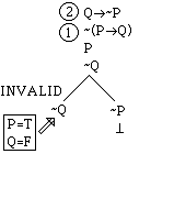
Now we will work out the tree for Q>-P | P>Q to see what happens with an invalid argument. We begin by writing down the premise and the negative of the conclusion:

Q>-P

-(P>Q)

Applying the rule for negative conditionals we obtain:

Now we apply the rule for positive conditionals to Q>-P:

Note that the right-hand branch contains a contradiction, so we mark it closed.

However, the left hand branch is still open. Since we have worked on every complex sentence, we have a full account of the possibilities for counterexamples for this argument. The left hand branch reports that there is a counterexample, namely one with P, -Q, and -Q all true. That amounts to saying that there is a counterexample with P = T and Q = F. We list this counterexample by putting the values in a box:

Here is a review of the tree construction process.

1. Write down the premises and the negative of the conclusion.

2. Apply tree rules to every complex sentence.

3. Mark every branch that contains a contradiction with ƒ.

4. If all branches are closed (contain ƒ), the argument is valid; if any branch is open (no ƒ on it), then this branch describes a counterexample and the argument is invalid.

Let's review the process with a more complex argument: (P&Q)>R, P | Q>R. First enter the premises and the negative of the conclusion:

(P&Q)>R

P

-(Q>R)

Now apply the negative conditional rule to the last line:

Now apply the positive conditional rule to the first premise:

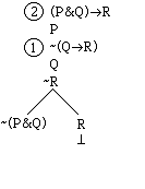
Notice that the right hand branch is closed because it contains -R and R, so we have marked it with ƒ. Now we must apply a rule to -(P&Q). The rule for negative conjunctions is similar to De Morgan's Law: -(A&B) | -Av-B. If A&B is F then either A is false or B is false:

Applying this rule to -(P&Q), we obtain:

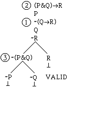
Since all branches close, the argument is valid.

There are still a few details about the tree method that need explaining. To illustrate, we will work out the tree for PvQ | P&Q. We begin entering the premise and negative conclusion as usual, and we have already applied the negative & rule to the last step:

Now we must work on PvQ. It is easy enough to see what rule we want here. If AvB is T then either A is T or B is T:

The problem is where to put the result of applying this rule. We have two open branches in our tree, one ending with -P and the other ending with -Q, and neither one is closed. So where do we place the new branch generated by PvQ:

on the left (below -P) or on the right (below -Q)? It would be wrong to do either one, and it would also be wrong to divide the results of applying the rule between the two sides like this:

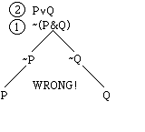
To see what we should do, it helps to remember what the tree represents. The two branches ending with -P and -Q represent two alternatives: for there to be a counterexample, either P = F or Q = F. However, the fact that PvQ is T means that on top of these two alternatives there are two more, either P = T or Q = T. So the correct thing to do is represent a total of four alternatives. Beneath the alternative -P, we need to record the alternative P or Q, and beneath -Q we must do so as well. This illustrates a basic principle about building a tree when there is more than one open branch.

The results of applying a rule to a line must be entered on every open branch below that line.

Following this principle, our tree now looks like this:

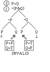
Note that contradictions appeared on two of the branches, so we marked them closed: Since we have worked on every step, the tree is complete and we can evaluate the argument. Note that there are two open branches indicating two different counterexamples to our argument. So the argument is invalid. It is a good idea to calculate the truth table for this argument to verify that it has these two counterexamples. One nice thing about trees is that they always give a full account of all the counterexamples to an argument.

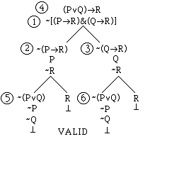
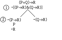
Our next project will be to show that (PvQ)>R | (P>R)&(Q>R) is valid using trees. We begin by negating the conclusion, and applying the negative & rule:

Next we will work on the -(P>R) on the left hand branch. According to the negative > rule we enter P and -R below -(P>R). It is not necessary to place P and -R below the right hand branch. Remember the rule is to put the results of applying a rule on every open branch below the formula you are working on.

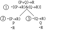
After working on -(Q>R) on the right branch, we obtain.

Now we will work on the first line: (PvQ)>R. In this case, we must place the result of applying the rule on all open branches below this line. So the result goes on both branches:

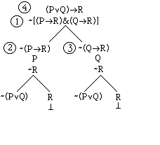
All that remains is to work on the -(PvQ) on each branch. The rule for a negative v is as follows:

-(AvB)

-A

-B

This rule is related to DeMorgan's Law. The idea is that when AvB is F, then both A and B are F. Applying this rule on each branch we complete the tree:

There is a final detail about tree construction worth mentioning. You may have been curious about the order in which I have carried out the steps in the trees. You might want to experiment with the problems we have already done to see what happens if you carry out the steps in a different order. In each case I have ordered the steps to keep the tree as simple as possible. There is a simple recipe to help economize in tree construction. The branching rules tend to create open branches, and subsequent steps must be copied onto all these open branches. For this reason, it is a good idea to do the non-branching steps first. Then when branching steps are finally carried out, there is a better chance that the branches created will close.

As a last note, we must discuss the <> rules. The rules may appear complex. But there is a simple way to remember them.

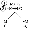
In case A<>|B is T, the values of A and B match. So either A and B are both T or A and B are both F. So the positive <> rule indicates these two possibilities on two branches. In case A<>B is F, then the values of A and B disagree. So either A is T and B is F or A is F and B is T. This is why the negative <> rule shows two alternatives, one containing A and -B and the other containing -A and B. Here is a tree for the argument M<>G | G<>M to help you practice these rules.

Since there are two open branches, the result of applying the negative <> rule to -(M<>G) goes on both sides:

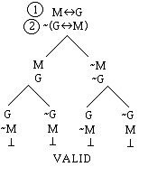
Note that all branches are closed. It is not necessary for there to be a contradiction for M and a contradiction for G to close a branch. One contradiction on a branch is enough to close it.