Lecture 15 (L/V predator/prey continued)
As we concluded from last lecture populations the Lotka/Volterra predator prey model results in a predictable manner called neutrally stable cycle.
The amplitude of the oscillation is simply dependent on the where the population starts.
If we relax some assumptions, e.g. add some density dependence, we can generate some realism in the model.
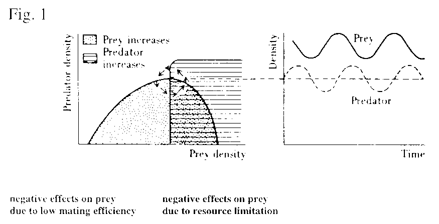
If the prey line and predation line are symmetrical this will lead to a stable limit cycle – returns to the same point.
Populations are rarely in such balance because natural selection favors predators becoming more efficient at capturing prey (especially if predator feeds on a single prey) and prey should be selected to decrease predator efficiency (escape mechanisms, etc.)
Predation does not decrease until prey levels are lower, i.e. they have a higher efficiency at capturing prey. Here predator can exploit prey very efficiently, vectors spiral outward leading to extinction of one or both species.
Called unstable cycle.
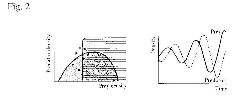
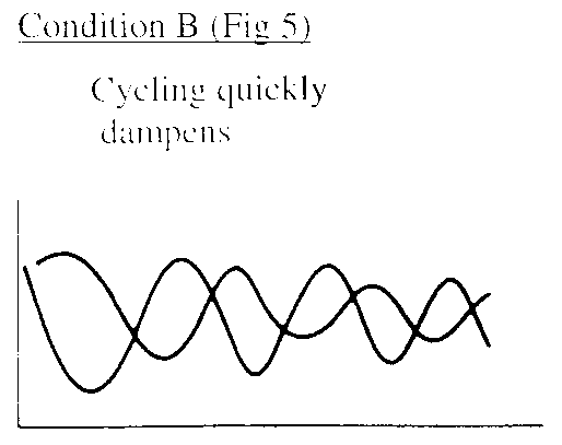
This situation will result in an inward spiraling of the cycle resulting in a dampened cycle. Predator and prey will tend to oscillate only slightly without perturbation.
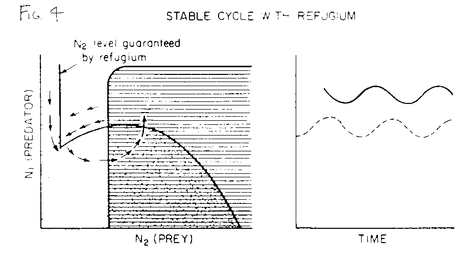
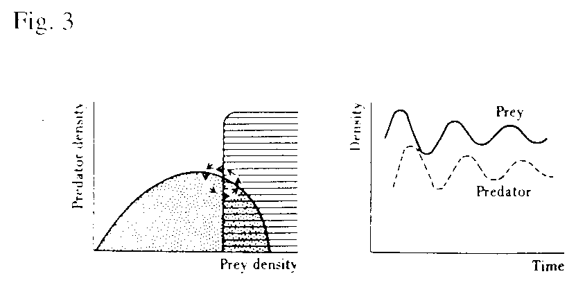
In this case prey have refuge where predators do not have access. Thus, any perturbation that destablizes the cycle can be restored by immigration.
Now let’s consider changes in the predator isocline:
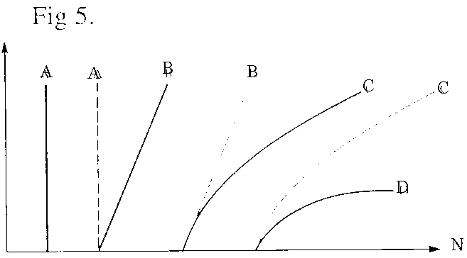
Fig 5.
Shift to the right at higher predator densities, more prey needed to increase predation density. Could be due to: 1) lower predation efficiency at high predator density because of social interactions (territoriality) leading to interference. Or, 2) mortality on predator is density-dependent. At higher densities predator mortality rate increases (outside effects).
Here A) L/V isocline, B) shows that more predators require more prey C) consumption rate is progressively reduced by mutual interference, D) predators limited by something other than food.
Consider: Condition B (Fig 5a)
Condition C (Fig 6)
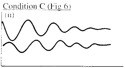
Finally, little cycling observed. Strong self-limitation. Predation intensity only high when population of predators is low and prey is near carrying capacity
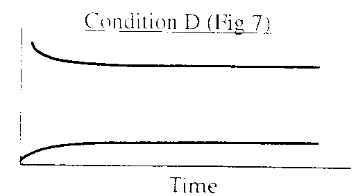
Condition D (Fig 7)
Why study the dynamics of predator/prey relationships ?
Intrinsically interesting in providing insight into the stability of natural systems.
But, also implication for successful management of human activities involved in exploiting natural resources.
The idea of managed harvesting is to maximize the crop yield (i.e. prey intake), while insuring that the prey does not go extinct.
From examples of our theoretical assessment of predator/prey cycling we found that coexistence is influenced by:
-refugia
-density-dependent effects on prey and predator
- switching
Unfortunately human attempts at conscious balancing to insure neither overexploitation nor under exploitation has not had a good record – e.g. collapse of cod fishery in North Atlantic.
Idea: Reducing population size will generally affect life-expectancy and fecundity of organisms.
However, How the population size is reduced is important is important to how population responses in number over time.
Controlled lab experiments showing density-dependent limitations on population growth also show that when adults are removed population growth is enhance because there is an excess of food for younger stages.
Results: high per capita increase in fecundity, increased birth rate (via reduced intraspecific competition).
So, act of harvesting will affect the rate of population growth.
Consider: Timing of harvest of cohort (e.g. Salmon)
Fig. 8
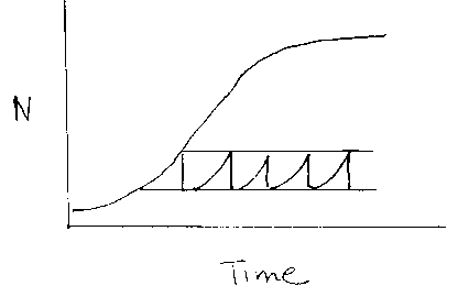
Fig. 9
harvest middle, pop. Growth period rapid, mix of adult and juvenile
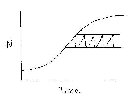
Fig. 10
harvest late, slow return (mostly adults)
Harvesting in middle of population considered optimum. Size and speed of recovery of population size are maximized Þ maximum sustained yield
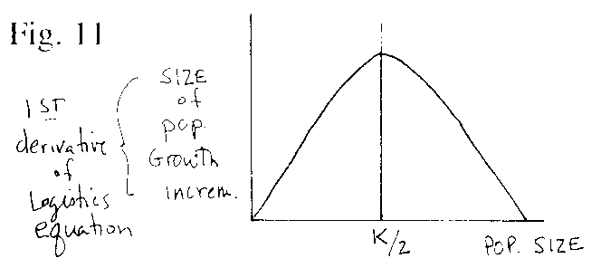
From the logistic equation, optimum population size to harvest in K/2.
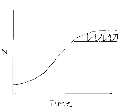
Fig. 11
Important point here is that maximum sustainable yield not obtained when population is at carrying capacity, although that may be the biggest "one-time" yield.
Maximum sustained yield is obtained at less than maximum population density.
Concept of maximum sustainable yield (MSY) is based on identification of "stock" – in practice it is a subset of the entire population, presumed to be representive of the entire "population"
Syear2 = Syear1 + R + G - D - C ;
S= stock @ time x
R= recruitment
G= growth
D= natural death
C= catch
To maintain this equality gains (R + G) must equal losses (D + C). C is maximized when population is at K/2.
Problems with early fishery models – assumed parameters were constant over time. If catch remains set at same limit but recruitment decreased
then overfishing results.
For example: many fisheries are characterized by populations that exist under "boom or bust" cycles resulting from environmental variability independent of human intervention.
Peru anchovy fishery 1955 –1972 catch reached maximum of 12 million tons/year.
Anchovy fishery is concentrated along central Chile to northern Peru. Spawning peaks Oct and February/March followed by recruitment in July/Sept.
Region characterized by periodic abrupt changes in sea surface temperature every 3-5 years due to ENSO. Peak of event occurs between December and July leading to failure in spawning and recruitment.
In 1972, strong ENSO lead to mass mortality. Survivors clumped into pockets of cool water. Fisherman continued to fish remnants of stock, subsequently populations declined to very low levels and continued fishing efforts lead to (C>>R).
ENSO’s 1973, 1977-78, 1982-83 yielded < 1 million tons/yr.
Bottom line: In natural predator prey systems interactions are reciprocal and mechanisms exist to reduce probability of destabilization, such as refugia, density-dependent effects, etc. If no compensatory mechanisms, either predator and/prey go extinct.
New management models try to take into account effects of human activity with year to year monitoring to try to take into account effects of natural catastrophes. Leads to very strict seasonal catches (e.g. salmon and herring).
Summarize:
To have Lotka-Volterra type stable limit cycle in a predator/prey relationship predators should be:
Factors that can lead to coexistence between predator and prey: some of which should lead to oscillations)
-spatial
- numerical (predator swamping)