Lecture 14 – Predator prey interactions
We can add another level of complexity to understanding patterns of foraging among predators.
This is the effect of patch use:
Define patch as : a discrete habitat or object where prey is distributed somewhat uniformly and separated from other prey which occur in other patches.
Again, another model by Charnov (1976), developed to describe the movement of predator from one patch to another. The model describes how long a predator should spend foraging in a patch. Model referred to as Optimal Patch Theory or Marginal Value Theorem.
In general: consumer (predator) should spend more time in higher profitable patches. As patch quality changes due to resource depletion (e.g. bees feeding on flower nectar, insectivorous birds) predator should leave to find another patch.
Question: When should the decision to switch to another patch occur?
Optimum residence time will maximize it’s overall energy intake during a bout of foraging. In doing so, it will maximize the average rate of energy intake for the bout as a whole.
Movement between patches assumes energy intake will be zero.
|

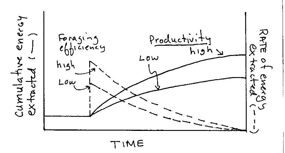
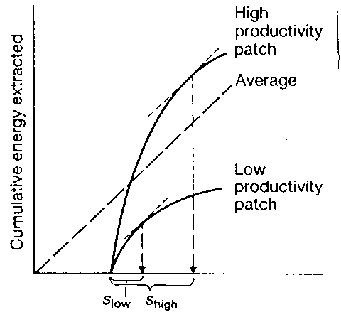
Graph 1.Cumulative energy extracted vs rate of extraction. |
Shape of curves are dependent on productively and foraging efficiency (i.e. amount of energy extracted/unit time)
Foraging efficiency higher ®
extraction rate is higher
Productivity higher ®
energy extracted is higher
|
Question: At what point should forager leave patch?
Extreme conditions
always moving, little time spent feeding. vs never move – deplete resource
therefore, some intermediate is optimal
Let’s consider:
- food is distributed patchily some patches more valuable than others.
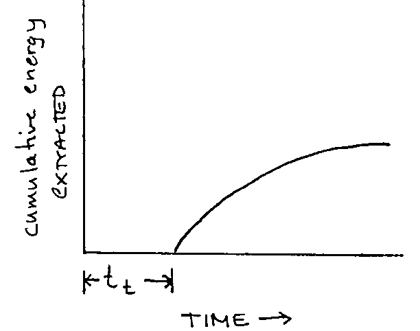
- average time spent travelling between patches is is tt. tt is the length of time a forager can expect to spend on average after leaving a patch before finding another.
|
Graph 2: Forager arrives in average patch:
 |
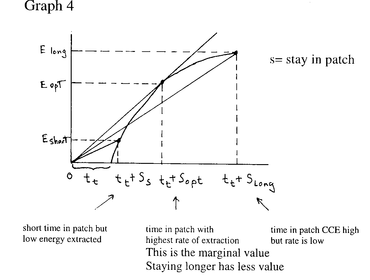
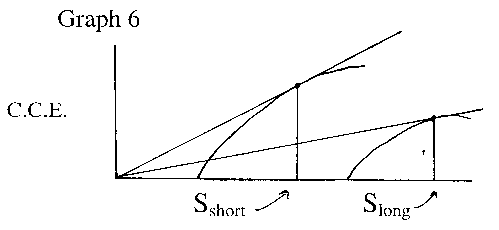
To forage optimally it must maximize it’s rate of energy intake not merely for its period in the patch but for the entire period since its departure from the last patch – period tt + S, S= duration in the patch.
|
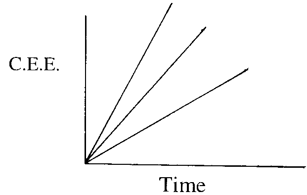
To maximize rate of energy extracted from the patch it will be a function of : cumulative energy extracted(CEE)/ time.
|
Graph 3 - Cumulative energy extracted (CEE) over time
Lines of equal reate of extraction

|

|
Some predictions generated from the marginal value theorem.
- Duration in the patch should be longer in more
productive habitats and shorter in less productive ones.
Graph 5 High productivity vs Low productivity
We assume rate of extraction same in habitats – extraction curves are parallel

|
Duration of stay longer when travelling time between patches is longer.

|
Predator/Prey cycles:
The population dynamics of predator/prey interactions.
Thus far we have considered population models which show how populations can be limited by resources (intraspecific interactions) and how interspecific competition can affect population size.
Do predators limit prey and vice-versa?
Sometimes clearly not, other times they appear to be tightly linked. In fact, some predator/prey systems show highly correlated oscillation patterns. Are these patterns due to direct interactions, or are they the result of indirect effects? Why are some systems stable and other not.
If predators do control prey populations and vice-versa, what are the conditions required to achieve that and is there any evidence for this?
Start with a simple model, then modify assumptions to see how predictions of the model change.
We’ll look at case studies to see if the model represents reality in nature.
Lotka- Volterra predation model
Model based on single predator-single prey relationship with three assumptions.
- Growth of the prey population is not restricted by the environment. Not realistic because most species have low population growth of very low densities and very high densities. For the first case (low) there is difficulty in finding mates, in the second case (high), food and/or space is limiting.
- The predators’ efficiency at capturing prey is constant
. Again, not realistic because most predators are better at capturing prey at certain densities (i.e. functional response changes).
- Population responses to increasing or decreasing growth in either the predator or prey is reasonably fast
. If not, predator can drive prey extinct or vice versa.
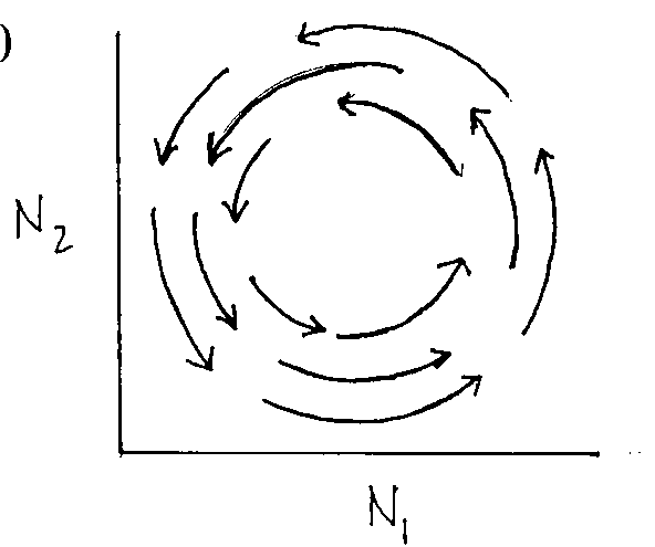
The predator-prey L/V model predicts that the predator and prey populations will oscillate in a periodic fashion – amplitude of oscillation dependent on initial size of the two populations. Any disturbance (external) will change the cycle amplitude. This type of system is referred to as being neutrally stable.
For the model:
N1 = number of individuals in prey population.
N2 = number of individuals in predator population
For prey:
y
1 = rate of removal of prey by predator
r1 = growth rate of prey population
y
1N2 = amount of prey removed by predator
To describe the rate of growth of the prey population:
dN1/dt = (r1 - y
1N2) N1
= (growth rate of prey - removal rate) (pop. of prey)
= r1 N1 -y
1N2 N1 where r1 and y
1 are constants
For predator:
birth rate of predator depends on density of prey so,
N1 = prey population
y
2 = efficiency of predator (in terms of converting
prey into predator offspring)
N1 y
2 = rate of increase of predator population
d2 = rate of death of predator
dN2/dt = (N1y
2 - d2) N2
(birth rate – death rate) x population size
= N2 N1y
2 - d2 N2
y
2 - d2 are constants
Like in the competition model, we can ask what population size will N1 and N2 be at equilibrium?
When dN/dt = 0
For prey:
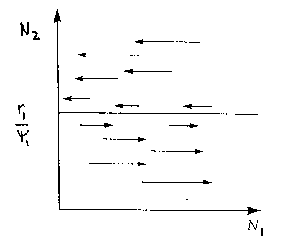
dN1/dt = 0 when N2 = r1/y
1 = rate of increase of prey/ rate of removal by predators
For predator:
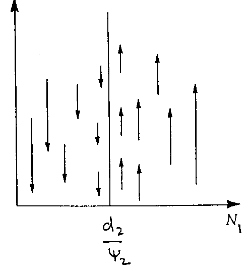
dN2/dt = 0 when N1 = d2/y
2 = rate of death predator/ rate of efficiency of predator
Now since r, d, and y
’s are constant these curves will be straight lines.
Model also assumes:
- no density-dependent regulation of predator or prey populations.
- environment is homogeneous.
- each prey has equal probability of being eaten.
- prey density does not affect the probability of prey item being eaten, i.e. type 1 functional response.
- predator density does not effect probability of predator catching a prey item.
|
So, for prey zero isocline (N1)
Graph 7

|
Above line predator removes prey past rate of replacement (prey decrease)
Below line predators remove prey slower than replacement rate (prey increase)
|
|
Graph 8
For predator zero isocline (N2)

|
If density of prey < d2/y
2, prey not sufficient to maintain
Population (predator decreases)
If prey > d2/y
2, the prey is higher than predator removal rate then predators increase.
|
|
Graph 10: Populations will cycle in predictable manner called neutrally stable cycle

|
N2 |
prey decrease (¬
)
predators decrease (¯
) |
prey decrease (¬
)
predators increase (
) |
|
prey increase (®
)
predators decrease (¯
) |
prey increase (®
)
predators increase (
) |
|
N1
Put them together: Graph 9 |
